You can locate the original blog post on observablehq.com, written by Herb Susmann.
Table of Contents
1. Functional
A functional (you could also call it a parameter) is any function that takes in a probability distribution and returns a number (or multiple numbers). For example, the mean is a functional: given a probability distribution, you compute $\mathbb{E}(X)=\int x p(x) d x$ and get back a number.
Mathematically, we can define the functional as $T(P):\mathscr{P} \rightarrow \mathbb{R}^q$, where ${\color{red}\mathscr{P}=\{P\}}$ is the family of the distributions.
A toy example
$$
T(P)=\int p(x)^2 d x\qquad(\star)
$$
This functional doesn’t usually have any practical significance
Other functionals might be
the average treatment effect in causal inference
the probability of survival after a certain time point in survival analysis.
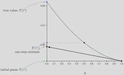
For the true data generating distribution $P$ (here, we can use $N(0,1)$), the value of this squared density parameter is $T(P)=0.282$.
However, we don’t know the true data generating distribution and we need to estimate it. Once we have an estimate of the distribution, we can “plug it in” to the formula for the functional to get an estimate for the parameter.
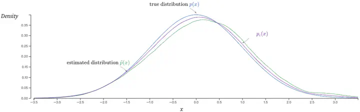
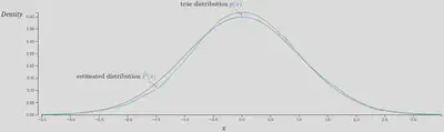
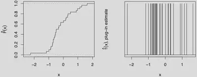
Take 100 samples from the true data generating distribution and use a kernel density estimator to obtain the estimated distribution $\tilde{P}$, with a corresponding density $\tilde{p}$. The following FIGURE shows how the estimated $\tilde{P}$ compares to the truth, $P$.
The difference between $\tilde{P}$ and the truth $P$
The estimate of the functional $(\star)$ using this estimated distribution is $T(\tilde P)=0.282$ (off by 1.5% compared to the true value).
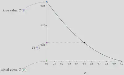
How would our estimate of the functional change if we could nudge our estimated distribution towards the true distribution ?
We define a family of distributions $P_\epsilon$ which are mixtures of the estimated distribution and the true distribution. The density of $p_\epsilon$ is given by
$$
p_\epsilon=(1-\epsilon) p+\epsilon \tilde{p}
$$
where $\epsilon\in[0,1]$. For every value of $\epsilon$ we can compute a corresponding value of the functional: $T\left(P_\epsilon\right)$. These values trace out a trajectory as they move from the initual guess, $T(\tilde{P})$, to the true value, $T(P)$, as shown in FIGURE below.
The difference between $\tilde{P}$ and the truth $P$
2. Pathwise Derivatives
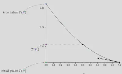
A pathwise derivative is the derivative of $T\left(P_\epsilon\right)$ with respect to $\epsilon$.
It’s useful to think of a derivative as a direction: for each value of $\epsilon$, the pathwise derivative tells us which direction the functional $T\left(P_\epsilon\right)$ is moving.
The pathwise derivative at $\epsilon=1$
When $\epsilon=1, \tilde{P}$ is the estimated distribution. The pathwise derivative at that point tells us how our estimate of $T(\tilde{P})$ would change if we nudged our estimate in the right direction, towards the true distribution.
3. One-step Estimator
We can use this to form a better estimate of the functional by using this pathwise derivative to approximate the trajectory as a linear function (shown in the following FIGURE). This is called a “one-step” estimator, because it’s like performing a single step of Newton’s method.
The one-step estimate
In any practical setting, we would need to use the observed data to estimate the pathwise derivative.
One-step estimators don’t respect any bounds on the target functional, which can lead to nonsensical results. An alternative family of estimators, Targeted Maximum Likelihood Estimators (TMLE), provide one way around this problem
4. Pathwise differentiability
A functional is called pathwise differentiable if it’s possible to compute it’s pathwise derivative.
This is a desirable property:
it allows for the creation of one-step estimators
it also allows for other techniques like Targeted Maximum Likelihood Estimation (TMLE).
Fortunately, many parameters of real-world interest are pathwise differentiable: for example:
the average treatment effect for a binary intervention is a pathwise differentiable parameter.
5. Influence function
The term influence function comes from its origins in robust statistics, where it was developed to quantify how much an estimator will change when its input changes (in other words, how much influence each input data point has on the outcome). In robust statistics, they’re mostly concerned with what happens when your data is perturbed in a bad direction, so they can understand how things like outliers will impact an estimator.
In our case, we are more interested in how estimators change when our estimates are nudged in the right direction, towards the true data distribution.
Is the plug-in estimator $T(\tilde F)$ a good estimator?
The Glivenko-Cantelli Theorem says that $\hat{F} \stackrel{\text { a.s. }}{\longrightarrow} F$; does this mean that $T(\hat{F}) \stackrel{\text { a.s. }}{\longrightarrow} T(F)$ ?
The answer turns out to be a complicated “sometimes”; often “yes”, but not always
The difference between $\tilde{P}$ and the truth $P$
When is the plug-in estimator consistent $\Rightarrow$ requires certain conditions on the smoothness
(differentiability) of $T(F)$ $\Rightarrow$ What does it mean to take the derivative of a function w.r.t. a function
5.1 The Gâteaux derivative
The Gâteaux derivative of $T$ at $F$ in the direction $G$ is defined by
$$
L_F(T ; G)=\lim _{\epsilon \rightarrow 0}\left[\frac{T\{(1-\epsilon) F+\epsilon G\}-T(F)}{\epsilon}\right]
$$
An equivalent way of stating the definition is to define $D=G-F$, and the above becomes
$$
L_F(T ; D)=\lim _{\epsilon \rightarrow 0}\left[\frac{T\{F+\epsilon D\}-T(F)}{\epsilon}\right]
$$
Either way, the definition boils down to
$$
L_F(T)=\lim_{\epsilon \rightarrow 0}\left[\frac{T\left(F_\epsilon\right)-T(F)}{\epsilon}\right]
$$
From a mathematical perspective, the Gâteaux derivative a generalization of the concept of a directional derivative to functional analysis
From a statistical perspective, it represents the rate of change in a statistical functional upon a small amount of contamination by another distribution $G$
An example: how the Gâteaux derivative work
Suppose $F$ is a continuous CDF, and $G$ is the distribution that places all of its mass at the point $x_0$. What happens to the Gâteaux derivative of $T(F)=f\left(x_0\right)$ ?
$$
\begin{aligned}
L_F(T ; G) & =\lim_{\epsilon \rightarrow 0}\left[\frac{\frac{d}{d x}{(1-\epsilon) F(x)+\epsilon G(x)}_{x=x_0}-\left.\frac{d}{d x} F(x)\right|_{x=x_0}}{\epsilon}\right] \\
& =\lim_{\epsilon \rightarrow 0}\left[\frac{(1-\epsilon) f\left(x_0\right)+\epsilon g\left(x_0\right)-f(x_0)}{\epsilon}\right] \\
& =\infty
\end{aligned}
$$
Conclusions:
Even though $F$ and $F_\epsilon$ differ from each other only infinitesimally $T(F)$ and $T\left(F_\epsilon\right)$ differ from each other by an infinite amount
The Glivenko-Cantelli theorem does not help us here: $\sup _x|\hat{F}(x)-F(x)|$ may go to zero without $T(\hat{F}) \rightarrow T(F)$
5.1.1 Hadamard differentiability
Gâteaux differentiability is too weak to ensure that $T(\hat{F}) \rightarrow T(F)$
Even if the Gâteaux derivative exists, it may not exist in an entirely unique way, and this is the subtle idea introduced by Hadamard differentiability
A functional $T$ is Hadamard differentiable if, for any sequence $\epsilon_n \rightarrow 0$ and $D_n$ satisfying $\sup _x\left|D_n(x)-D(x)\right| \rightarrow 0$, we have
$$
\frac{T\left(F+\epsilon_n D_n\right)-T(F)}{\epsilon_n} \rightarrow L_F(T ; D)
$$
If $T$ is Hadamard differentiable, then $T(\hat{F}) \stackrel{\mathrm{P}}{\longrightarrow} T(F)$
5.1.2 Bounded functionals
Another useful condition: if the functional is bounded, then the plug-in estimate will converge to the true value
Proposition: Suppose that there exists a constant $C$ such that the following relation holds for all $G$ :
$$
|T(F)-T(G)| \leq C \sup _x|F(x)-G(x)|.
$$
Show that $T(\hat{F}) \stackrel{\text { a.s. }}{\longrightarrow} T(F)$.
5.2 The influence function
5.2.1 Contamination by a point mass
The idea of contaminating a distribution with a small amount of additional data has a long history in statistics and the investigation of robust estimators. Statisticians usually do not work with the general Gâteaux derivative, but a special case of it called the influence function, in which $G$ places a point mass of 1 at $x$ :
$$
\delta_x(u)= \begin{cases}0 & \text { if } u<x \\ 1 & \text { if } u \geq x\end{cases}
$$
5.2.2 Influence function & empirical influence function
The influence function is usually written as a function of $x$, and defined as
$$
L(x)=\lim_{\epsilon \rightarrow 0}\left[\frac{T\left\{(1-\epsilon) F+\epsilon \delta_x\right\}-T(F)}{\epsilon}\right]
$$
A closely related concept is that of the empirical influence function:
$$
\hat{L}(x)=\lim _{\epsilon \rightarrow 0}\left[\frac{T\left\{(1-\epsilon) \hat{F}+\epsilon \delta_x\right\}-T(\hat{F})}{\epsilon}\right]
$$
Example: if $T(F)=\mu$, then we have $L(x)=x-\mu$ and $\hat L(x)=x-\bar x$
5.2.3 Linear functionals
A functional $T(F)$ is a linear functional iff $T(F)=\int a(x) d F(x)$. For the linear functionals, we have
$$
\begin{aligned}
& L(x)=a(x)-T(F) \\
& \hat{L}(x)=a(x)-T(\hat{F})
\end{aligned}
$$
Example: if $T(F)=\sigma^2$, then we have $L(x)=(x-\mu)^2-\sigma^2$ and $\hat L(x)=(x-\bar x)^2-\hat\sigma^2$
References
Visually Communicating and Teaching Intuition for Influence Functions (Fisher & Kennedy 2020)