On factor models with random missing: EM estimation, inference, and cross validation

$$ \begin{aligned} \ \end{aligned} $$

Outline

• Background: factor model
• Motivation
• Factor models with random missing:
  • EM estimator
  • Asymptotic properties
  • Determining the number of factors
• Simulation
• Empirical application

Background: factor model

$$ \begin{aligned} x_{i t} & =\lambda_i f_t+e_{i t} \\ \boldsymbol{X} &= \boldsymbol{\Lambda} \boldsymbol{F}^\top + \boldsymbol{E} \end{aligned} $$

• $\boldsymbol{X}=(\boldsymbol{x}_{\cdot 1},\ldots,\boldsymbol{x}_{\cdot T})\in\mathbb{R}^{N\times T}$

• $\boldsymbol{\Lambda}\in\mathbb{R}^{N\times R}$: factor loadings

• $\boldsymbol{F}\in\mathbb{R}^{T\times R}$: common factors (latent, unobserved)

• $\boldsymbol{E}\in\mathbb{R}^{N\times T}$: idiosyncratic (or error) component

  • ${e_{it}}$ can exhibit both cross-sectional and temporal dependence.

• Given the factor number $k$, we can estimate the factors and factor loadings by $$ \Big\{\widehat{\boldsymbol{\Lambda}}^k, \widehat{\boldsymbol{F}}^k\Big\}=\arg\min_{\boldsymbol{\Lambda}^k,\boldsymbol{F}^k}\frac{1}{NT}\Big\|\boldsymbol{X}- \boldsymbol{\Lambda}^k{\boldsymbol{F}^k}^\top\Big\|_F^2 $$ where $\boldsymbol{\Lambda}^k\in\mathbb{R}^{N\times k}$ and $\boldsymbol{F}^k\in\mathbb{R}^{T\times k}$.

Motivation

• Factor model in balanced panel has been thoroughly investigated. $$$$
• How to handle the missing data problem in factor models? $$$$
  • the expectation–maximization (EM) algorithm $$$$
  • the Kalman filter (KF) $$$$
• There is no formal study of the asymptotic properties for the EM estimators of the factors and factor loadings for the PC estimation with missing observations

Notations

• consider the factor model $$ \boldsymbol{X} = \boldsymbol{F}\boldsymbol{\Lambda}^\top + \varepsilon $$

  • $\boldsymbol{X}=(X_1,\ldots,X_N)$ where $X_i \equiv\left(X_{i 1}, \ldots, X_{i T}\right)^{\prime}$ and $X_{it}$ are missing at random
  • $\varepsilon=\left(\varepsilon_1, \ldots, \varepsilon_N\right)$ and $\varepsilon_i \equiv\left(\varepsilon_{i 1}, \ldots, \varepsilon_{i T}\right)^{\prime}$ for $i=1, \ldots, N$.
  • $F=\left(F_1, \ldots, F_T\right)^{\prime}$ and $\Lambda=\left(\lambda_1, \ldots, \lambda_N\right)^{\prime}$ where $F_t$ and $\lambda_i$ are $R \times 1$ vectors of factors and factor loadings

• $F^0=\left(F_1^0, \ldots, F_T^0\right)^{\prime}$ and $\Lambda^0=\left(\lambda_1^0, \ldots, \lambda_N^0\right)^{\prime}$ are the true values of $F$ and $\Lambda$

• $\Omega \subset[N] \times[T]$ be the index set of the observations that are observed. That is, $$ \Omega=\Big\{(i, t) \in[N] \times[T]: X_{i t} \text { is observed }\Big\}. $$

• Let $G$ denote a $T \times N$ matrix with $(t, i)$ th element given by $g_{i t}=\mathbf{1}\{(i, t) \in \Omega\}$ and is independent of $X, F^0, \Lambda^0$ and $\varepsilon$

The initial estimates

• Let $\tilde{X}=X \circ G$ and $\tilde{X}_{i t}=X_{i t} g_{i t}$.

• The common component $C^0 \equiv F^0 \Lambda^0$ is a low rank matrix $\Rightarrow$ it is possible to recover $C^0$ even when a large proportion of elements in $X$ are missing at random.

• Under the standard condition that $E\left(\varepsilon_{i t} \mid F_t^0, \lambda_i^0\right)=0$, we can verify that $E\left(\frac{1}{q} \tilde{X} \mid F^0, \Lambda^0\right)=F^0 \Lambda^{0 \prime}$ $\Rightarrow$ consider the following least squares objective function $$ \mathcal{L}_{N T}^0(F, \Lambda) \equiv \frac{1}{N T} \operatorname{tr}\left[\left(\frac{1}{\tilde{q}} \tilde{X}-F \Lambda^{\prime}\right)\left(\frac{1}{\tilde{q}} \tilde{X}-F \Lambda^{\prime}\right)^{\prime}\right] $$ identification restrictions: $F^{\prime} F / T=I_R$ and $\Lambda^{\prime} \Lambda$ is a diagonal matrix.

• By concentrating out $\Lambda$ and using the normalization that $F^{\prime} F / T=I_R$ $\Rightarrow$ identical to maximizing $\tilde{q}^{-2} \operatorname{tr}\Big\{F^{\prime} \tilde{X} \tilde{X}^{\prime} F\Big\}$

The initial estimates

• The estimated factor matrix, denoted by $\hat{F}^{(0)}$ is $\sqrt{T}$ times the eigenvectors corresponding to the $R$ largest eigenvalues of the $T \times T$ matrix $\frac{1}{N T \tilde{q}^2} \tilde{X} \tilde{X}^{\prime}:$ $$ \frac{1}{N T \tilde{q}^2} \tilde{X} \tilde{X}^{\prime} \hat{F}^{(0)}=\hat{F}^{(0)} \hat{D}^{(0)}, $$
  • $\hat{D}^{(0)}$ is an $R \times R$ diagonal matrix consisting of the $R$ largest eigenvalues of $\left(N T \tilde{q}^2\right)^{-1} \tilde{X} \tilde{X}^{\prime}$, arranged in descending order along its diagonal line.
• The estimator of $\Lambda^{\prime}$ is given by $$ \hat{\Lambda}^{(0) \prime}=\frac{1}{\tilde{q}}\left(\hat{F}^{(0) \prime} \hat{F}^{(0)}\right)^{-1} \hat{F}^{(0) \prime} \tilde{X}=\frac{1}{T \tilde{q}} \hat{F}^{(0) \prime} \tilde{X} . $$
• We can obtain an initial estimate of the $(t, i)$ th element, $C_{i t}^0$, of $C^0$ by $\hat{C}_{i t}^{(0)}=\hat{\lambda}_i^{(0)\prime} \hat{F}_t^{(0)}$.
• The initial estimators $\hat{F}_t^{(0)}, \hat{\lambda}_i^{(0)}$ and $\hat{C}_{i t}^{(0)}$ are consistent and follow mixture normal distributions under some standard conditions.

The iterated estimates

• The initial estimators: consistency but not asymptotically efficient $\Rightarrow$ iterative estimators
• In step $\ell$, we can replace the missing values $\left(X_{i t}\right)$ in the matrix $X$ with the estimated common components $\hat{C}_{i t}^{(\ell-1)}$. Define the $T \times N$ matrix $\hat{X}^{(\ell)}$ with its $(t, i)$ th element given by $$ \hat{X}_{i t}^{(\ell)}=\left\{\begin{array}{ll} X_{i t} & \text { if }(i, t) \in \Omega \\ \hat{C}_{i t}^{(\ell-1)} & \text { if }(i, t) \in \Omega_{\perp} \end{array}, \ell \geq 1,\right. $$ where $\Omega_{\perp}=\{(i, t) \in[N] \times[T]:(i, t) \notin \Omega\}$.
• Then we can conduct the PC analysis based on $\hat{X}^{(\ell)}$ and obtain $\hat{F}^{(\ell) \prime}$ and $\hat{\Lambda}^{(\ell)}$.
• We will study the asymptotic properties of $\hat{F}_t^{(\ell)}, \hat{\lambda}_i^{(\ell)}$ and $\hat{C}_{i t}^{\left(\ell^{\ell}\right)}, \ell=1,2, \ldots$

$$ ~\\\ ~\\\ $$

Asymptotic properties of the initial estimators

Theorem 2.1. Suppose some assumptions hold. Then $$\frac{1}{T}\Big\|\hat{F}^{(0)}-F^0 \hat{H}^{(0)}\Big\|_F^2=O_P\left({\color{red}\delta_{N T}^{-2}}\right)$$ where $\delta_{N T}=\sqrt{N} \wedge \sqrt{T}$.

• $\hat{H}^{(0)}$ is defined as $$ \hat{H}^{(0)}=\left(N^{-1} \Lambda^{0 \prime} \Lambda^0\right) T^{-1} F^{0 \prime} \hat{F}^{(0)}\left(\hat{D}^{(0)}\right)^{-1}, $$ where $\hat{D}^{(0)}$ is asymptotically nonsingular by Lemma A.1.

Asymptotic distributions

Theorem 2.2. Suppose some assumptions hold. Suppose that $\left(T^{1 / 2}+N^{1 / 2}\right) \delta_{N T}^{-2}=o(1)$. Let $\hat{\Pi}_{t N}^{(0)}=\sqrt{N}\Big(\hat{F}_t^{(0)}-\hat{H}^{(0) \prime} F_t^0\Big)$ and $\hat{\Pi}_{i T}^{(0)}=\sqrt{T}\Big(\hat{\lambda}_i^{(0)}-(\hat{H}^{(0)})^{-1} \lambda_i^0\Big)$. Then as $(N, T) \rightarrow \infty$

1. $\hat{\Pi}_{t N}^{(0)}=\Big(\hat{D}^{(0)}\Big)^{-1} \frac{1}{T} \hat{F}^{(0) t} F^0 \frac{1}{\sqrt{N} q} \sum_{i=1}^N \lambda_i^0 \xi_{i t}+O_P\Big(N^{1 / 2} \delta_{N T}^{-2}\Big) \rightarrow N\Big(0, D^{-1} Q \Gamma_{g, t}(q) Q^{\prime} D^{-1}\Big) \mathcal{G}^t$-stably,
2. $\hat{\Pi}_{i T}^{(0)}=\hat{H}^{(0) \prime} \frac{1}{\sqrt{T} q} \sum_{t=1}^T F_t^0 \xi_{i t}+O_P\left(T^{1 / 2} \delta_{N T}^{-2}\right) \rightarrow N\left(0,\left(Q^{\prime}\right)^{-1} \Phi_{g, i}(q) Q^{-1}\right) \mathcal{G}^i$-stably,
3. $\Big(\frac{1}{N} \Sigma_{F, i t}^{(0)}(q)+\frac{1}{T} \Sigma_{\Lambda, i t}^{(0)}(q)\Big)^{-1 / 2}\Big(\hat{C}_{i t}^{(0)}-C_{i t}^0\Big) \stackrel{d}{\rightarrow} N(0,1)$,

Asymptotic properties of the iterated estimators

Theorem 2.3. Suppose some assumptions hold. Then $$\frac{1}{T}\Big\|\hat{F}^{(\ell)}-F^0 \hat{H}^{(\ell)}\Big\|^2=O_P\left(\delta_{N T}^{-2}\right)$$ for each $\ell$, where $\hat{H}^{(\ell)}$ is defined as $$ \hat{H}^{(\ell)}=\left(N^{-1} \Lambda^{0 \prime} \Lambda^0\right) T^{-1} F^{0 \prime} \hat{F}^{(\ell)}\Big(\hat{D}^{(\ell)}\Big)^{-1}, $$

Asymptotic distributions

Theorem 2.4. Suppose some assumptions hold. Suppose that $\sqrt{N}\big(T^{\gamma_1 / 4} \delta_{N T}^{-2} \ln T+T^{-1+3 \gamma_1 / 4}\big)=o(1)$ and $\sqrt{T}\big(N^{\gamma_2 / 4} \delta_{N T}^{-2} \ln N+N^{-1+3 \gamma_2 / 4}\big)=o(1)$. Let $\hat{\Pi}_{t N}^{(\ell)}=\sqrt{N}\Big(\hat{F}_t^{(\ell)}-\hat{H}^{(\ell) \prime} F_t^0\Big)$ and $\hat{\Pi}_{i T}^{(\ell)}=\sqrt{T}\Big(\hat{\lambda}_i^{(\ell)}-\hat{H}^{(\ell)-1} \lambda_i^0\Big)$. Then

• $\hat{\Pi}_{t N}^{(\ell)}=D^{-1} Q \frac{1}{\sqrt{N}} \sum_{i=1}^N \lambda_i^0 \varepsilon_{i t} g_{i t}+(1-q) \hat{\Pi}_{t N}^{(\ell-1)}+o_P(1)$ uniformly in $t$ and $$ \hat{\Pi}_{t N}^{(\ell)} \stackrel{d}{\rightarrow} N\left(0, D^{-1} Q {\color{red}\Gamma_{1 g, t}(q)} Q^{\prime} D^{-1}\right) \text { as }(\ell, N, T) \rightarrow \infty $$
• $\hat{\Pi}_{i T}^{(\ell)}=\left(Q^{\prime}\right)^{-1} \frac{1}{\sqrt{T}} \sum_{t=1}^T F_t^0 \varepsilon_{i t} g_{i t}+(1-q) \hat{\Pi}_{i T}^{(\ell-1)}+o_P(1)$ uniformly in $i$ and $$ \hat{\Pi}_{i T} \stackrel{d}{\rightarrow} N\left(0,\left(Q^{\prime}\right)^{-1} {\color{red}\Phi_{1 g, i}(q)} Q^{-1}\right) \text { as }(\ell, N, T) \rightarrow \infty, $$
• $\left(\frac{1}{N} \Sigma_{1 F, i t}+\frac{1}{T} \Sigma_{1 \Lambda, i t}\right)^{-1 / 2}\left(\hat{C}_{i t}^{(\ell)}-C_{i t}^0\right) \stackrel{d}{\rightarrow} N(0,1)$ as $(\ell, N, T) \rightarrow \infty$.

Determining the number of factors via CV

• Given the $T \times N$ matrix of observations $X$:
  • randomly sample elements in $X$ with a fixed probability $p \in(0,1)$
  • leave the rest $(1-p)$-proportion of observations as held-out entries for the out-of-sample evaluation.
• Let $\Omega^\star \subset[N] \times[T]$ be the index set of the training entries and $\Omega_{\perp}^\star$ the index set of the held-out entries.
• Define the operator $P_{\Omega^\star}: \mathbb{R}^{T \times N} \rightarrow \mathbb{R}^{T \times N}$ by $$ \left(P_{\Omega^\star} X\right)_{t i}=X_{i t} g_{i t}^\star=X_{i t} \mathbf{1}\left\{(i, t) \in \Omega^\star\right\}, $$ where $g_{i t}^\star=\mathbf{1}\left\{(i, t) \in \Omega^\star\right\}$.
• Let $G^\star$ denote a $T \times N$ matrix with $(t, i)$ th element given by $g_{i t}^\star$.
• Now we can regard $P_{\Omega^\star} X$ as the $T \times N$ data matrix with missing values replaced by zeros.

Determining the number of factors via CV

• Given $P_{\Omega^\star} X$, we apply the proposed EM algorithm to recover the data via estimating the common component matrix $C$ for any given number of factors.
• To proceed, we consider the full singular value decomposition (SVD) for $\frac{1}{p} P_{\Omega^\star} X$: $$ \frac{1}{p} P_{\Omega^\star} X=\tilde{U} \tilde{\Sigma} \tilde{V}^{\prime}=\sum_{r=1}^{T \wedge N} \tilde{u}_r \tilde{v}_r^{\prime} \tilde{\sigma}_r, $$
  • $\tilde{U}\in\mathbb{R}^{T \times T}=\left(\tilde{u}_1, \ldots, \tilde{u}_T\right)$
  • $\tilde{V}\in\mathbb{R}^{N \times N}=\left(\tilde{v}_1, \ldots, \tilde{v}_N\right)$
  • $\tilde{\Sigma}\in\mathbb{R}^{T \times N}$ is the diagonal matrix that contains the singular values, $\tilde{\sigma}_1, \tilde{\sigma}_2, \ldots, \tilde{\sigma}_{T \wedge N}$, arranged in descending order along the main diagonal line.
• Given any $R \leq T \wedge N$ and the training entries in $P_{\Omega^\star} X$, we can estimate the common component $C$ by the singular value thresholding procedure: $$ \tilde{C}_R=S_H\left(\frac{1}{p} P_{\Omega^\star} X, R\right)=\tilde{U}_R \tilde{\Sigma}_R \tilde{V}_R^{\prime}=\sum_{r=1}^R \tilde{u}_r \tilde{v}_r^{\prime} \tilde{\sigma}_r, $$ where $S_H(\cdot, R)$ is the rank-R truncated SVD of $\cdot$, t

Determining the number of factors via CV

• Let $\tilde{C}_{R, i t}$ denote the $(t, i)$ th element of $\tilde{C}_R$ for $R \geq 1$.
• We propose to choose $R$ to minimize the following CV criterion function $$ {\color{red}\widetilde{C V}(R)=\frac{1}{N T} \sum_{(i, t) \in \Omega_{\perp}^\star}\left[X_{i t}-\tilde{C}_{R, i t}\right]^2.} $$
• Let $\tilde{R}=\arg \min _{0 \leq R \leq R_{\max }} \widetilde{C V}(R)$ where $R_{\max }$ is a fixed integer that is no less than $R_0$

$$ ~\\\ ~\\\ ~\\\ ~\\\ ~\\\ $$

A more efficient method

• Can we use the $\ell$-step estimator $\hat C_{R,it}^{(\ell)}$ ?
• Suppose that we have obtained the estimates $\hat{C}_{R, i t}^{(\ell-1)}$. In step $\ell$, we can replace the zero elements in $X^\star \equiv P_{\Omega^\star} X$ with the estimated common components $\hat{C}_{R_{\max }, i t}^{(\ell-1)}$
• Define the $T \times N$ matrix $\hat{X}^{\star(\ell)}$ with its $(t, i)$ th element given by $$ \hat{X}_{i t}^{\star(\ell)}= \begin{cases}X_{i t} & \text { if }(i, t) \in \Omega^\star \\ \hat{C}_{R_{\max }^{(\ell-1)}}, & \text { if }(i, t) \in \Omega_{\perp}^\star, \ell \geq 1,\end{cases} $$ where $\Omega_{\perp}^\star=\big\{(i, t) \in[N] \times[T]:(i, t) \notin \Omega^\star\big\}$
• Conduct the singular value thresholding procedure: $$ \hat{C}_R^{(\ell)}=S_H\big(\hat{X}^{*(\ell)}, R\big)=\hat{U}_R^{(\ell)} \hat{\Sigma}_R^{(\ell)} \hat{V}_R^{(\ell) \prime}, $$
• repeating the above procedure for $\ell=1, \ldots, \ell^\star \equiv\left\lfloor\ln \left(\epsilon_{N T}\right) / \log (p)\right\rfloor$
• Let $\hat{C}_R=\hat{C}_R^{(\ell^\star)}$ and $\hat{R}=\arg \min _{0 \leq R \leq R_{\max }} \widehat{C V}(R)$, where $$ \widehat{C V}(R)=\frac{1}{N T} \sum_{(i, t) \in \Omega_{\perp}^\star}\left[X_{i t}-\hat{C}_{R, i t}\right]^2 $$

The consistency of the CV method

Assumption A.7.

1. For $r=R_{0+1}, \ldots, R_{\max }, \\ P\Big(\big\|\tilde{u}_r\big\|_{\infty}\big\|\tilde{v}_r\big\|_{\infty} \leq 1 /\big(c_0 \sqrt{(N+T) \log (N+T)}\big)\Big) \rightarrow 1$ for some fixed $c_0<\infty$ as $(N, T) \rightarrow \infty$, $\left\|\tilde{u}_r\right\|_{\infty}=o_P(1)$, and $\left\|\tilde{v}_r\right\|_{\infty}=o_P(1)$
2. $\max _{(i, t) \in \Omega_{\perp}^\star} \sum_{(j, s) \in \Omega_{\perp}^\star}\left|E\left[\varepsilon_{i t} \varepsilon_{j s} \mid P_{\Omega^\star} X, \Omega^\star\right]\right|=o_P\left(\delta_{N T}^2\right)$.

Theorem 3.1. Suppose some assumptions hold. Then $P\left(\tilde{R}<R_0\right) \rightarrow 0$ as $(N, T) \rightarrow \infty$. If Assumption A.7 also holds, then $P\left(\tilde{R}>R_0\right) \rightarrow 0$ as $(N, T) \rightarrow \infty$.

Theorem 3.2. Suppose some assumptions hold. Then $P\left(\hat{R}<R_0\right) \rightarrow 0$ as $(N, T) \rightarrow \infty$. If Assumption A.7 also holds, then $P\left(\hat{R}>R_0\right) \rightarrow 0$ as $(N, T) \rightarrow \infty$.

CV in the presence of random missing

• Consider the SVD for $\frac{1}{p \tilde{q}} P_{\Omega^\star} P_{\Omega} X$ : $$ \frac{1}{p \tilde{q}} P_{\Omega^\star} P_{\Omega} X=\tilde{U} \tilde{\Sigma} \tilde{V}^{\prime}, $$
• Then we estimate the common component $C$: $$ \tilde{C}_R=S_H\left(\frac{1}{p \tilde{q}} P_{\Omega^\star} P_{\Omega} X, R\right)=\tilde{U}_R \tilde{\Sigma}_R \tilde{V}_R^{\prime}, $$ where $\tilde{U}_R, \tilde{V}_R$, and $\tilde{\Sigma}_R$ are defined as before. Let $\tilde{R} \in\big\{0,1,2, \ldots, R_{\max }\big\}$ minimize the following $\mathrm{CV}$ function $$ \widetilde{C V}(R)=\frac{1}{N T} \sum_{(i, t) \in {\color{red}\Omega_{\perp}^\star \cap \Omega}}\left[X_{i t}-\tilde{C}_{R, i t}\right]^2, $$

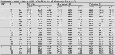
Simulation

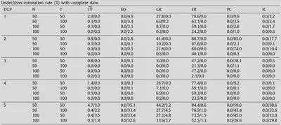
Simulation

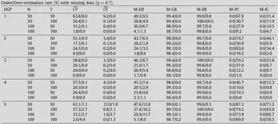
Simulation

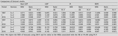
Empirical application: Forecasting macroeconomic variables

• We use a panel dataset FRED-QD, which is an unbalanced panel at the quarterly frequency.
• The dataset consists of 248 quarterly U.S. indicators from 1959Q1 to 2018Q2.
• Use 125 time series to estimate the latent factors.
• Consider the forecast based on the following factor-augmented autoregression (FA-AR) models: $$ y_{t+h}^h=\phi_h^{(1)}+\phi_h^{(2)}(L) \hat{F}_t+\phi_h^{(3)}(L) y_t+\varepsilon_{t+h}^h, h=1,2,4, $$
  • $y_t$ is one of the four macro-variables (i.e., RGDP, GDP, IP, and RDPI)
  • $\hat{F}_t$ is the estimated vector of factors
  • $\phi_h^{(1)}$ is the intercept term, $L$ is the lag operator
  • $\phi_h^{(2)}(L)$ and $\phi_h^{(3)}(L)$ are finite-order polynomials of the lag operators

Empirical application: Forecasting macroeconomic variables

Thanks !